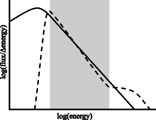
| (6.1) |
| (6.2) |
| (6.3) |
| (6.4) |
| Dte | power law exponent | |
| upstream | downstream | |
| 0.1 We-1 | -1.73 | -1.93 |
| 0.05 We-1 | -2.07 | -2.16 |
| 0.025 We-1 | -2.06 | -2.18 |
| 0.0125 We-1 | -1.96 | -2.02 |
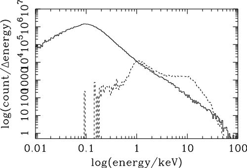
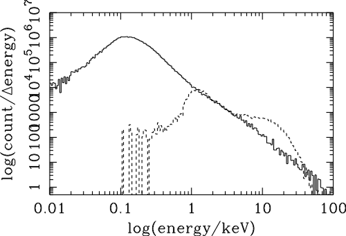
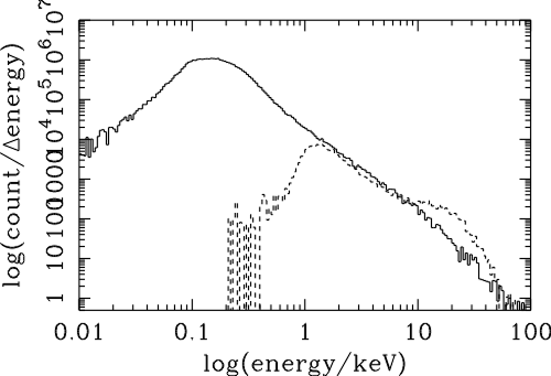
| Vin | qBn | MA | �B1 �/B0 | �B2 �max/B0 | Var(Bx)/B0 | Eesc(a = 180�) |
| 1.4 vA | 88� | 2.68 | 2.22 | 2.25 | 0.00238 | 60 eV |
| 2 vA | 80� | 3.30 | 2.79 | 2.70 | 0.0469 | 3.5 eV |
| 2 vA | 85� | 3.34 | 2.80 | 2.66 | 0.0198 | 15 eV |
| 2 vA | 88� | 3.35 | 2.76 | 2.63 | 0.0290 | 94 eV |
| 2 vA | 89� | 3.35 | 2.79 | 2.67 | 0.0163 | 380 eV |
| 4 vA | 80� | 5.65 | 4.55 | 3.87 | 0.689 | 11 eV |
| 4 vA | 85� | 5.67 | 4.54 | 3.93 | 1.01 | 43 eV |
| 4 vA | 88� | 5.67 | 4.67 | 3.86 | 1.14 | 270 eV |
| 4 vA | 89� | 5.68 | 4.49 | 3.71 | 1.30 | 1.1 keV |
| 6 vA | 88� | 8.21 | 6.12 | 3.95 | 3.35 | 570 eV |
| Vin | tinit | tfinal | upstream boundary |
| 1.4vA | 15 Wi-1 | 37.5 Wi-1 | x � -25 vA Wi-1 |
| 2vA | 15 Wi-1 | 37.5 Wi-1 | x � -25 vA Wi-1 |
| 4vA | 10 Wi-1 | 37.5 Wi-1 | x � -25 vA Wi-1 |
| 6vA | 10 Wi-1 | 27.0 Wi-1 | x � -10 vA Wi-1 |